
Relevance, Probative Value, and Preponderance of the Evidence
Introduction
Here we’ll discuss the relevance and probative value of an item offered as evidence to prove an asserted fact. We’ll also discuss what it means to prove a fact under the preponderance standard of proof. To do this, we’ll think about these evidence issues in terms of
- the probability that the offered item of evidence exists, given a world in which the fact sought to be proven is true; and
- the probability that the fact to be proven is true, given the offered item of evidence.
Here’s some motivation. In everyday speech, it’s tempting to use vague words like “weak”, “strong”, or “a lot” to denote how much proof of an alleged fact you have or whether you have enough to meet your burden of production on that issue. But that vagueness leads to muddy thinking, particularly as the disputed facts become more complex. It also makes it easier to confuse the two probability statements above (sometimes called the “prosecutor’s fallacy” – a mislabel because any lawyer can make that mistake).
There is a better way. What follows is a gentle introduction to ways of thinking about evidence that simplifies a complex conceptual literature on evidence and probability in law (for reviews, see Ho 2021; Urbaniak and Di Bello 2021). Don’t worry if you find it hard or non-intuitive at first. The key is to follow the illustrative examples slowly and carefully, step by step, and to ask me questions about the bits that are elusive.
Background
If a legal rule requires proving an alleged fact, a judge or jury (the fact-finder) must decide whether there is enough evidence to take that fact as proven true. The answer is either “yes” or “no”. No hedging (“Well, it might be true . . .”) allowed!
But what counts as enough evidence for a court that the fact is true? That depends on the applicable standard of proof. In civil cases (e.g. tort lawsuits) in the US, that is typically called the “preponderance of the evidence” standard.
This means that when a judge or jury declares a finding of fact, it isn’t saying that the alleged fact is true or not. Rather, it declares a fact to be proven true or not, given the items of evidence somebody actually offered up (and a court admitted) and a standard of proof that sets how much evidence is enough before the factfinder may decide to take that fact as proven true.
What counts as proof? To prove an alleged fact, lawyers look to three main items:
- exhibits admissible under the rules of evidence (e.g., photos, documents, objects)
- sworn witness testimony admissible pursuant to the rules of evidence
- stipulated facts, i.e., facts that the parties expressly agree to take as true
The first two items on this list depend on whether a trial judge agrees that the offered item is admissible under the rules of evidence. Every State court has its own rules of evidence, and the federal courts follow the Federal Rules of Evidence. When an item is admitted as evidence, that item is placed into the court record. (Think of the “record” as a really big box of stuff.)
In turn, all the items of evidence in the court record are for the fact-finder (the judge or jury) to weigh when deciding whether an alleged fact in the case has been proven true. An item’s admissibility doesn’t say anything about its weight. For example, the testimony of an alleged eyewitness may be admissible, but the jury may decide to assign zero weight to that evidence, because it believes that the witness is lying. Nor does it matter how many items of evidence in the record there are. Remember, factfinders are not supposed to count the number of items of evidence; rather, they weigh items of evidence individually and cumulatively.
Let’s start thinking about evidence issues in terms of probability statements. To do this, we’ll start with a non-law problem (medical testing), and then turn to a problem in a legal setting.
NoteWhat’s a Probability?
A probability denotes the degree of plausible belief in any proposition \(X\), given what you already know or assume (\(\mathcal{I}\)). For example, if X = Eight planets orbit our sun, then \(Pr(X \mid \mathcal{I})\) is shorthand for the how much you can plausibly believe that Eight planets orbit our sun is true, given what you know or take as true about planets, our solar system, and other background assumptions.
Here, we’ll be talking about the probability of propositions for there are two mutually exclusive and exhaustive possibilities: it is true (\(X\)) or not true (\(\lnot X\)).
Any probability is expressed as a number between 0 and 1 (e.g. \(P(X \mid \mathcal{I})\) = 0.25), with “0” denoting certainly false and “1” denoting certainly true. We can equivalently express that probability as a percentage, e.g., 25% ; a fraction (=\(\frac{25}{100} = \frac{1}{4}\)); and a frequency (“25 out of 100”).
We can also convert a probability into odds and vice-versa. For any probability \(p\) of a proposition \(X\), the corresponding odds of \(X\) is \(\frac{p}{1 - p}\). For example, a probability of 0.25 equals an odds of \(\frac{0.25}{1 - 0.25} = \frac{1}{3}\). Conversely for any odds of \(X\), the corresponding probability \(p = \frac{\text{odds}}{1 + \text{odds}}\). So, an odds of \(\frac{1}{3}\) equals a probability of \(\frac{\frac{1}{3}}{\frac{4}{3}} = 0.25\). This will be useful later.
Example: Medical Testing
Suppose you are a physician and consider this problem:
The probability of breast cancer is 1% for a woman at age 40 who participates in routine screening. If a woman has breast cancer, the probability is 80% that she will receive a positive mammography. If a woman does not have breast cancer, the probability is 9.6% that she will also receive a positive mammography. A woman in this age group had a positive mammography in a routine screening. What is the probability that she actually has breast cancer?
To solve this problem, let’s break it down into its key parts:
Identify the reference class \(\mathcal{I}\). Here, the reference class is “women at age 40 who participate in routine screening.” For any reference class we select, we make some background assumptions. Here, that can include what causes them to get breast cancer.
The first number (1%) describes the probability that someone in the reference class truly has breast cancer, that is, \(P(X | \mathcal{I}) = 0.01\). This probability is sometimes called the ‘prevalence’ or ‘base rate’.
The second number (80%) is the probability that the mammography (E) detects breast cancer if someone in the reference class truly has that cancer, i.e., \(P(E\mid X,\mathcal{I})=0.80\). This is the mammography test’s true positive rate (sometimes called its ‘sensitivity’). The test’s false negative rate (the test says “no cancer” when the person in fact has it) is just one minus its true positive rate (here, 20%).
The third number (9.6%) is the probability that the mammography indicates breast cancer even though the person in fact does not have breast cancer. This probability (\(P(E\mid\lnot X,\mathcal{I}))=0.096\)) is the test’s false positive rate. The mammography test’s true negative rate (sometimes called its ‘specificity’) is just one minus the false-positive rate (here, 0.904).
Translate into Frequencies
You’ve been asked for the probability that a woman in this reference class has cancer, given a positive mammography test result, or \(P(X \mid E,\mathcal{I})\). To do this, let’s now translate the given information into frequencies.
Imagine that the reference class \(\mathcal{I}\) (“women at age 40 who participate in routine screening”) consists of 1,000 people.
Now, divide up these 1,000 people into two subsets: those with breast cancer and those without breast cancer. We’ve been told that 1% of these women have breast cancer. That’s the same as saying out of these 1,000 women, 10 will have breast cancer, because 1% of 1000 = \(\frac{10}{1000}\). This means that the other 990 women (\(=1000 - 10\)) do not have breast cancer.
Next, divide up the women with breast cancer. The mammography’s true-positive rate of 80% indicates that out of the 10 women with breast cancer, 8 (because 80% = \(\frac{8}{10}\)) will be detected by a mammography and the other 2 women with breast cancer (\(=10-8\)) will be missed by this test.
Similarly, divide up the women without breast cancer. According to the mammography’s false-positive rate of 9.6%, out of the 990 women who truly do not have breast cancer, the mammography will erroneously classify 95 of them as having breast cancer (because 9.6% of 990 \(\approx 95\)) and correctly classify the other 895 women (\(=990-95\)) has not having breast cancer.
Visualization with Icon Array
It is easier to see all this by depicting these calculations with pictures and diagrams. One approach is the icon array.
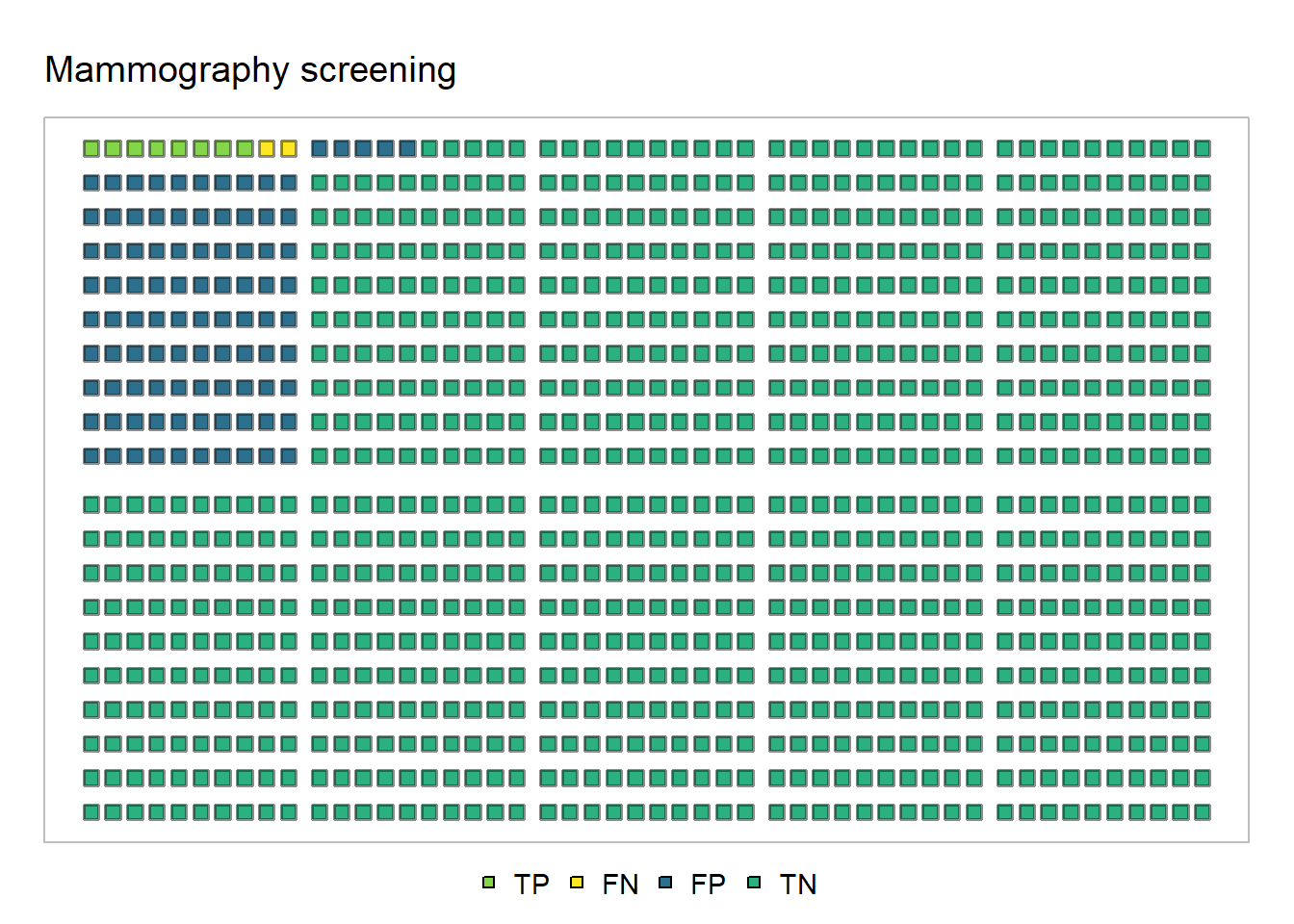
In the array depicted in Figure 1, there are 1,000 squares, and each square represents a person.
The light-green squares (
TPfor true positive) are the (8) people that the mammography indicates breast cancer and actually do have breast cancer.The dark-green squares (
TNfor true negatives) are the (895) people that the mammography indicates no breast cancer and actually do not have breast cancer.The blue squares (
FPfor false positives) are the (95) people that the mammography indicates breast cancer but actually do not have breast cancer.The yellow squares (
FNfor false negatives) are the (2) people that the mammography indicates not breast cancer but actually do have breast cancer.
Using this array, let’s now ask: “How many of the women with a mammogram indicating breast cancer actually have breast cancer?” To answer this question, find the number of women with a mammogram indicating breast cancer by counting the number of blue squares and the number of light-green squares. (I’ll wait.)
Did you get 103, i.e., \(= 8 + 95\)? Good. Now, of those 103, how many actually have breast cancer? You already know this – it’s the number of light-green squares alone, i.e., the number of true positives. So, the answer is \(\frac{8}{103} \approx 7.8\%\).
Visualization with Tree Diagram
Because icon arrays can be a pain to draw, another approach is the tree diagram. Think of the tree branches in Figure 2 as depicting how we divided up our population of 1,000 people above.
For a dynamic variation on the tree diagram, check out the pachinkogram (Budgett and Pfannkuch 2021).
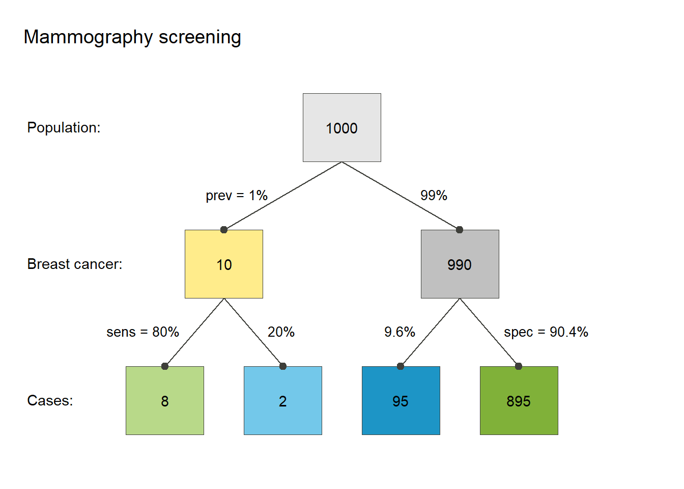
Let’s now ask: “How many of the women with a positive mammogram actually have breast cancer?” From the bottom row of tree diagram, we know that 103 (\(= 8 + 95\)) women obtained a positive result on a mammography (total positives = true positives + false positives). Out of these, however, only 8 truly have breast cancer, that is, are true positives. Therefore, the probability of actually having breast cancer, given a positive mammography result, is \(\frac{8}{8+95} = \frac{8}{103} \approx 7.8\%\).
Thus, given a positive mammography result, someone from our reference class (“women at age 40 who participate in routine screening”) has only a 7.8% probability of actually having breast cancer. This is so low, even though mammography accurately detects breast cancer 80% among women in this reference class. Why? Because in our reference class, breast cancer is so rare overall (1%).
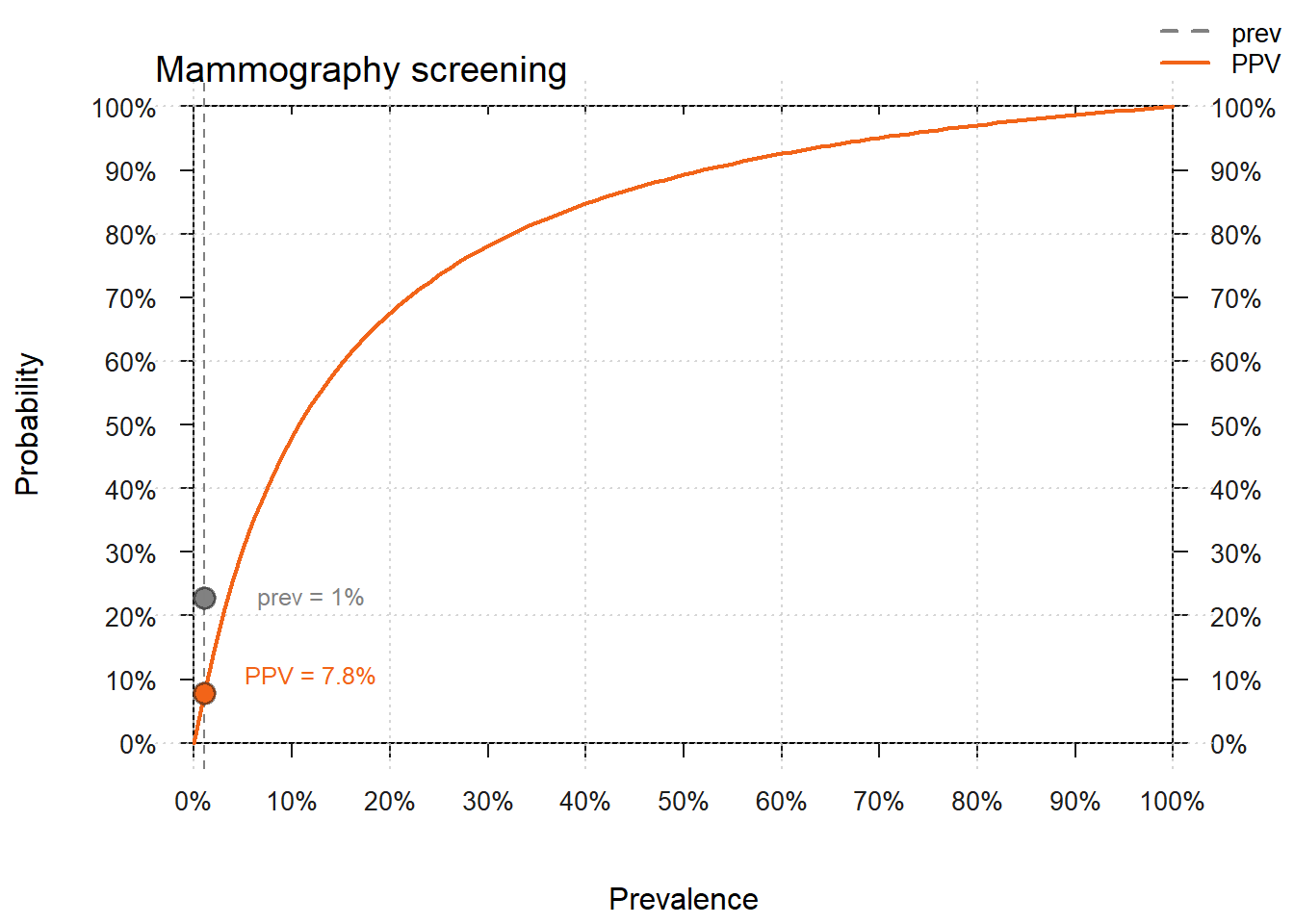
Figure 3 depicts how (assuming zero uncertainty) as breast cancer prevalence (its base rate) increases in the reference class, the true-positive probability (PPV) increases as well.
Example: Who Shot the Plaintiff?
Okay, what does this have to do with evidence in a lawsuit? By similar reasoning, we can now generate, for a lawsuit, probability statements that match up with the relevance and probative value of an item of evidence, as well as (arguably) whether the evidence, taken alone, suffices to prove the alleged fact under the preponderance standard of proof.
To see how, consider this problem.
Suppose you bring a tort lawsuit against a defendant, your client’s roommate, for accidentally shooting your client with a gun. Your client did not see who shot him, but strongly believes that it was the defendant, who was his roommate at the time. The roommate denies this, but you have discovered that he kept a gun in their shared apartment.
Based on your research into gunshot cases like this, you believe and can show the following:
In cases like these, we start with prior belief, based on background knowledge or a set of assumptions, that the probability of getting shot by a household member is 15%, i.e., \(P(X\mid\mathcal{I}) = 0.15\)
If someone in these kinds of cases truly did get shot by a household member, the probability is 80% that someone in that person’s household will have kept a gun in that household, that is, \(P(E | X,\mathcal{I}) = 0.80\).
If someone in these kinds of cases truly did not get shot by a household member (\(\lnot X\) is true), the probability is 9.6% that someone in that person’s household will have kept a gun in that household, i.e., \(P( E | \lnot X,\mathcal{I}) = 0.096\).
As a lawyer, if you have to persuade the jury that the defendant shot your client, you may also have to persuade the trial judge
To admit an item of evidence (here, that the defendant kept a gun in the household) as relevant to proving that critical fact
That your item of evidence also has enough probative value to satisfy any other rule of law for which probative value matters.
That this item of evidence, along with the other items admitted as evidence, is enough for a reasonable jury to find that the defendant (the roommate) shot your client under the preponderance of the evidence standard of proof. (You might have to argue this in a motion filed before a trial, during a trial, or after a verdict.)
Let’s take on each of these now.
Relevance
What is relevance? If we are in federal court, we’d turn to Federal Rule of Evidence 401:
Evidence is relevant if: (a) it has any tendency to make a fact more or less probable than it would be without the evidence; and (b) the fact is of consequence in determining the action.
Fed. R. Evid. 401. Most States have a similar evidence rule. E.g., Connecticut Code of Evidence \(\S\) 4-1.
Applied here, Federal Rule of Evidence 401 means that the evidence (E = Defendant kept a handgun in the household) counts as “relevant” if that evidence is more or less likely to exist in a world where the defendant really did shoot the plaintiff (X) than in a world where, all else equal, the defendant really did not shoot the plaintiff (\(\lnot X\)).
One way to express this idea is with the likelihood ratio (LR):
\[LR = \frac{P(E | X, \mathcal{I})}{P(E | \lnot X, \mathcal{I})}\] Thus, when we say that an item of evidence \(E\) has “any tendency to make a fact more or less probable than it would be without the evidence,” we mean it must satisfy this condition:
\[\frac{P(E | X, \mathcal{I})}{P(E | \lnot X, \mathcal{I})} \neq 1\].
In words, if the evidence is equally likely to exist in cases like this in a world where the roommate truly shot the plaintiff and in another otherwise equal world where the roommate didn’t shoot the plaintiff, that evidence is by definition not relevant. To illustrate, if the evidence is testimony that the defendant ate nachos last week, that evidence is irrelevant if that nachos-eating is no more or less likely to occur for cases from the reference class in which the roommate was the shooter and cases in which the roommate was not the shooter.
Note
In practice, lawyers often dispute an alleged fact by offering an alternative story of what happened. Here, the defendant’s lawyer might dispute that that the defendant is the shooter by pointing to somebody else (Dr. Richard Kimble) as the “real” shooter. To use the likelihood ratio in this situation, just take the two options (\(X_1\) = defendant as shooter; \(X_2\) = Kimble as shooter) as mutually exclusive and exhaustive of the possibilities. Then, \(LR = \frac{P(E | X_1, \mathcal{I})}{P(E | X_2, \mathcal{I})}\). In words, this expresses how likely it is that the defendant kept a gun in the household in a world where he is the shooter as compared to a world in which Kimble is the shooter, assuming that these are the only possibilities and both cannot have occurred.
Here, the evidence is relevant: \(LR = \frac{.80}{.096} = \frac{25}{3} \neq 1\). As a result, that item of evidence may be admissible because it is relevant, unless it fails to satisfy some other kind of law. E.g. Fed. R. Evid. 402.
Warning
Don’t confuse relevance with the question of how likely the evidence is to exist if the disputed fact is true. To see why, suppose that an item of evidence is 30% likely in a world where he shot the gun, and 25% likely in a world where the roommate is not the shooter. Thus, in both worlds, the evidence is unlikely to exist, that is, \(P(E \mid X, \mathcal{I}) < 0.50\) and \(P(E \mid \lnot X, \mathcal{I}) < 0.50\). Is the item of evidence still relevant? Yes, because \(LR = \frac{.30}{.25} \neq 1\). Or in words, even though both possibilities are unlikely, the item of evidence still gives us some information about which of those two worlds we are in.
Probative Value
An item of evidence’s probative value often refers to how much weight to assign that item of evidence in deciding whether an alleged fact is true.
One intuitive approach is to take an item of evidence’s likelihood ratio to indicate its probative value. If LR = 1 for an item of evidence, it has zero weight. We assign more weight depending on how much the LR exceeds one. And if LR < 1, the item of evidence has weight, but for the proposition that X is not true. In our example, the item’s LR \(= \frac{.80}{.096}= 8\frac{1}{3}\).
Even when lacking precise values for the constituent probabilities, forensic scientists and others use the idea of a likelihood ratio when testifying in court as to the weight of the evidence (Nordgaard and Rasmusson 2012).
Probative value can matter for admissibility. Consider, for example, Federal Rule of Evidence 403:
The court may exclude relevant evidence if its probative value is substantially outweighed by a danger of one or more of the following: unfair prejudice, confusing the issues, misleading the jury, undue delay, wasting time, or needlessly presenting cumulative evidence.
Fed. R. Evid. 403. For the parallel rule in Connecticut, see Connecticut Code of Evidence \(\S\) 4-3.
Does Federal Rule of Evidence 403 mean that an item of evidence can be both relevant and inadmissible because its “probative value” is less than the danger that it’ll impose, say, “unfair prejudice” on a party? (“‘Unfair prejudice’ within its context means an undue tendency to suggest decision on an improper basis, commonly, though not necessarily, an emotional one.” Advisory Committee’s Notes on Fed. R. Evid. 403, 28 U.S.C. App., p. 860.) Yep. Cool, right?
Warning
Where there are multiple items of evidence, each item’s probative value may depend on the other admissible items of evidence (\(E_{1}, E_{2}, E_{3} . . .\)) that the plaintiff has offered to prove the same alleged fact. To illustrate, whatever the probative value of proof that the defendant kept a gun in the house, it might have less value if there is also an otherwise admissible signed statement by the defendant confessing to the shooting. Put another way, given that signed statement, the item of evidence that the defendant kept a gun in the house, though still relevant, might have a lower marginal probative value, because \(\mathcal{I}\) now includes the existence of that signed statement.
Preponderance of the Evidence
The “preponderance of the evidence” standard of proof typically applies to civil litigation in the U.S., which includes contract and tort lawsuits. The other two main standards of proof are the “reasonable doubt” standard, which applies in criminal proceedings, and the “clear and convincing” standard.
One way of translating the “preponderance” standard is that it requires the factfinder to believe that the material facts are “more likely than not” to be true, given the evidence in the record. Thus, in the simplest case, if the entire case depends on whether a single fact is true (\(X\)) or not true (\(\lnot X\)), the factfinder must decide for the plaintiff if the probability that the fact is true, given the evidence, is greater than fifty percent, that is, \(P(X | E,\mathcal{I})) > 0.50\).
Jury instructions, however, tend mostly to communicate standards of proof with words only (e.g, “more likely than not”). They don’t also provide an explicit probability formulation (e.g., “‘Preponderance’ means that, on a scale of 0% (not at all certain) to 100% (completely certain), you must be at least 51% certain of the truth of the plaintiffs’ case before you give a verdict in favor of the plaintiffs.”). This practice persists, despite research suggesting that quantified instructions do better than a words-only instruction in communicating the required degree of belief (e.g., Kagehiro 1990).
In any event, now let’s return to our hypothetical case to see if the evidence there meets the preponderance standard. To do this, we’ll proceed in three separate and valid approaches: (1) the frequency tree; (2) the icon array; and (3) calculating the posterior odds. While I recommend the tree approach, I’ll walk through all three approaches, which vary mostly in how easy they are to use and understand.
Frequency Tree
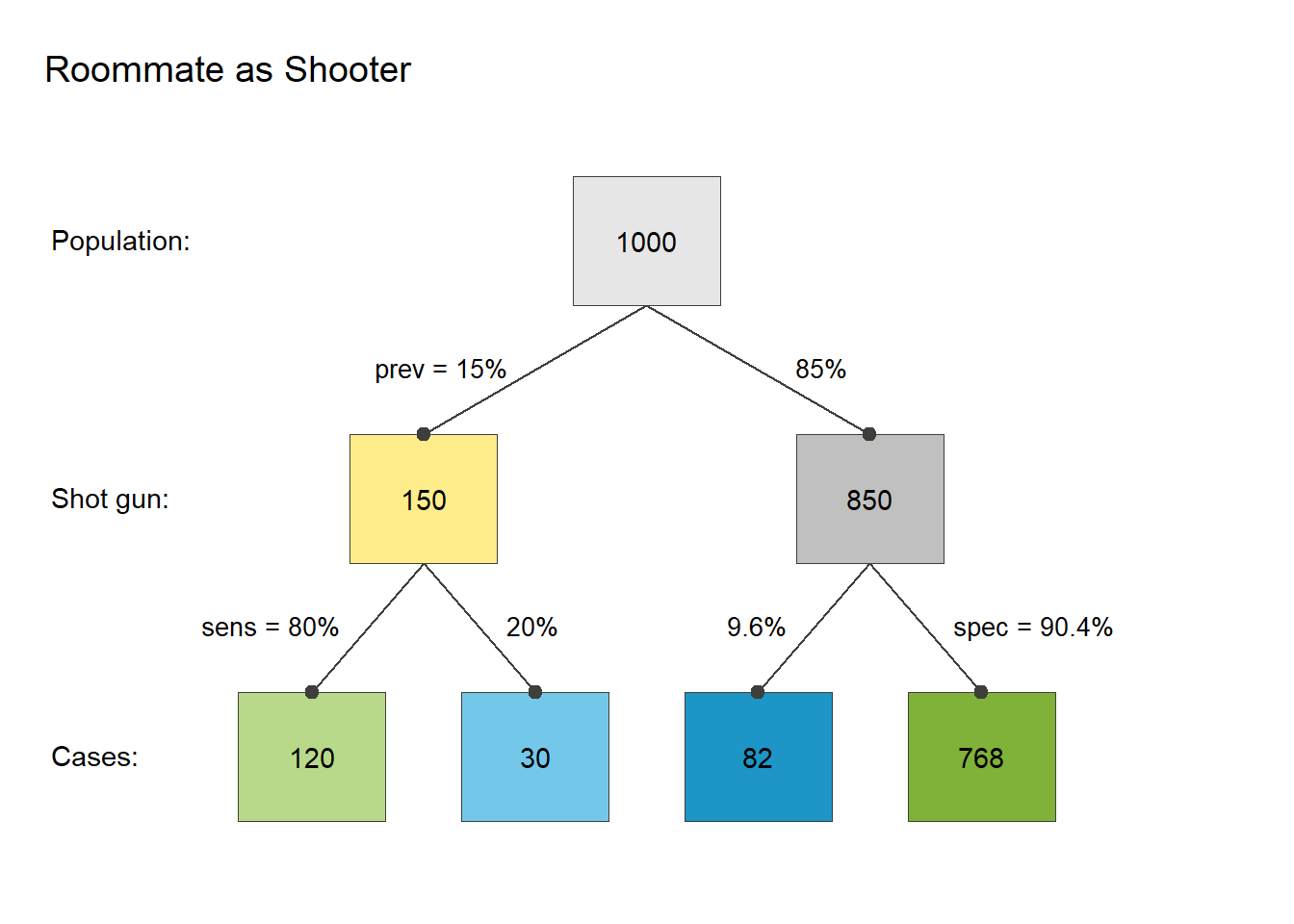
Suppose you start by assuming that \(P(X\mid\mathcal{I})= 0.15\). That’s like saying that you believe that out of, say, 1,000 cases like this one, 150 of them will be ones in which the household member was the shooter, because 15% of 1000 \(=\frac{150}{1000}\). This means no household shooter in the other 850 cases.
Next, divide up our population of cases as follows.
The true-positive rate of 80% indicates that of the 150 cases with a household shooter, 120 of them (80% = \(\frac{120}{150}\)) have evidence of a gun kept in the household and the other 30 cases there was no such evidence.
The false-positive rate of 9.6% indicates that out of the 850 cases without a shooter in the household, about 82 household members (9.6% \(\approx \frac{82}{850}\)) will be erroneously classified as the shooter if we rely only on whether they kept a gun in the house.
Now we have all we need to yield the following tree diagram (Figure 4):
From the tree diagram, let’s now answer the question: Given our assumptions, how likely is it that the defendant-roommate was the shooter?
We know that 202 (\(= 120 + 82\)) cases had proof of a gun kept in the house. Out of these, only 120 truly were cases with a household shooter. Therefore, the probability of a household shooter, given that there is a gun kept in the house, is \(\frac{120}{120+82} = \frac{120}{202} = 59.4\%\)
So, is proof that the defendant-roommate kept the gun in the house enough to support a verdict against the defendant under the “preponderance” standard of proof? Yes, because \(P(X \mid E,\mathcal{I}) \approx 0.59\), which is greater than fifty percent.
TipIcon Array
Here is an icon array for the same example.
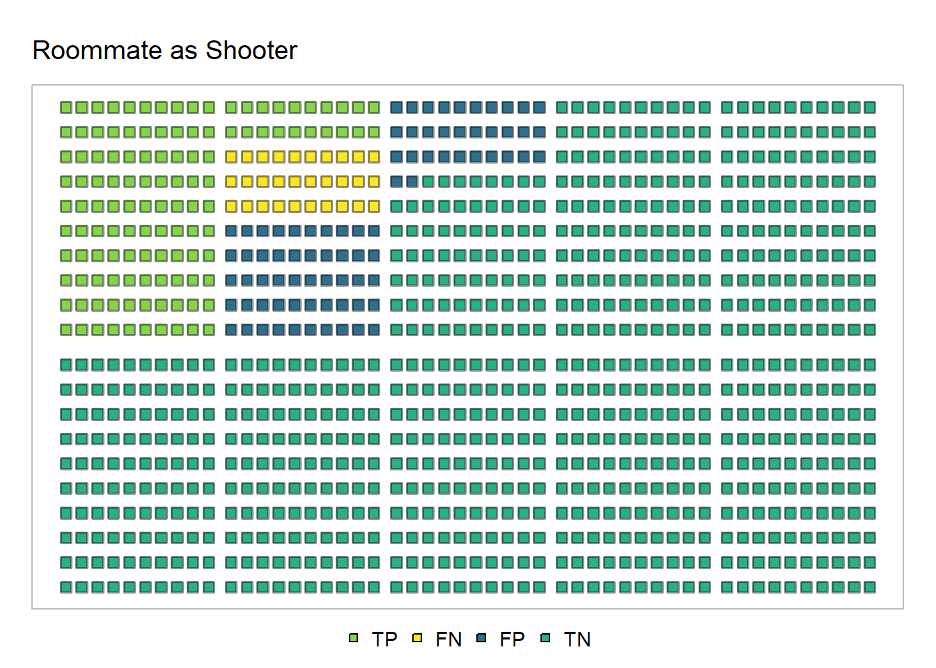
In the array depicted in Figure 5, there are 1,000 squares, and each square represents a case in the reference class.
The light-green squares (
TPfor true positive) are the cases where the defendant-roommate kept the gun and where that defendant truly was the shooter.The dark-green squares (
TNfor true negatives) are the cases where the defendant-roommate didn’t keep a gun and was not the shooter.The blue squares (
FPfor false positives) are the cases where defendant-roommate kept the gun but actually was not the shooter.The yellow squares (
FNfor false negatives) are the cases where the defendant-roommate didn’t keep a gun but actually was the shooter.
Did you get \(\frac{120}{120+82} \approx 59.4%\)?
TipPosterior Odds
For a more mathy approach, we could calculate the posterior odds, i.e.,
\[\text{Posterior Odds} = \text{Likelihood Ratio} \times \text{Prior Odds}\]
\[ \frac{P(X \mid E,\mathcal{I})}{P(\lnot X \mid E,\mathcal{I})} = \frac{P(E \mid X,\mathcal{I})}{P(E \mid \lnot X,\mathcal{I})} \times \frac{P(X\mid\mathcal{I})}{P(\lnot X\mid\mathcal{I})}\]
Okay, that’s a bit ugly. But actually, you’ve seen the component parts before. The prior odds is just the base rate expressed as odds. Here, that’s just \(\frac{0.15}{1 - 0.15} = \frac{15}{85} = \frac{3}{17}\). And you’ve already encountered the likelihood ratio, which here is \(\frac{.80}{.096} = \frac{25}{3}\).
Accordingly, the posterior odds is \(\frac{3}{17} \times \frac{25}{3} = \frac{75}{51}\) = 1.4705882. In words, this is just saying that, given the evidence, it is now 1.4705882 times more likely than not that the roomate is the shooter.
Finally, convert the posterior odds back to a probability. Just as a probability \(p\) can be expressed as odds \(\frac{p}{1 - p}\), we can convert an odds \(z\) into a probability \(\frac{z}{1 + z}\)
Here, \(Pr (X \mid E,\mathcal{I}) = \frac{1.470588}{1 + 1.470588} \approx 0.595\). In words, given the evidence, we should now treat as more plausible our belief that the roommate shot the gun from 15 percent - what we assumed before we considered the evidence - to about 59 percent. That’s pretty close to what you got with the other approaches. And it leads to the same conclusion that the “preponderance” standard is satisfied.
Test Your Intuitions
Now, test your intuitions by answering the following questions:
If you were a juror in this case, and liability depended only on proving that the defendant was the shooter, would you rule against the defendant and force him to pay damages to the plaintiff? Why?
If you were the trial judge in this case, and the jury found for the plaintiff, would you agree with a post-verdict motion to set aside the verdict on the ground that the evidence in the record was insufficient to show that that the defendant shot the plaintiff? Why?
If you answered “No” to at least one of those questions, is your concern about finding liability based on “statistical evidence” alone? If so, why? For discussion, see, e.g., Ross (2021).
Conclusion
Here, we discussed the relevance and probative value of an item offered as evidence to prove an asserted fact. We also discussed what it means to prove a fact under the preponderance standard of proof. To do this, we translated the legal rules into different kinds of probability statements and, to apply the preponderance standard, used primarily tree diagrams to infer one probability statement from another.
Colophon
All figures were produced with R version 4.5.3 (2026-03-11 ucrt) (R Core Team 2025) and the riskyr package (Neth et al. 2025).
References
Budgett, Stephanie, and Maxine Pfannkuch. 2021. Pachinkogram: Conditional Probabilities Visualisation. https://www.stat.auckland.ac.nz/~vt/.
Ho, Hock Lai. 2021. “The Legal Concept of Evidence.” In The Stanford Encyclopedia of Philosophy, Winter 2021, edited by Edward N. Zalta. Https://plato.stanford.edu/archives/win2021/entries/evidence-legal/; Metaphysics Research Lab, Stanford University.
Kagehiro, Dorothy K. 1990. “Defining the Standard of Proof in Jury Instructions.” Psychological Science 1 (May): 194–200. https://doi.org/10.1111/j.1467-9280.1990.tb00197.x.
Neth, Hansjoerg, Gaisbauer Felix, Gradwohl Nico, and Gaissmaier Wolfgang. 2025. Riskyr: Rendering Risk Literacy More Transparent. Social Psychology; Decision Sciences, University of Konstanz. https://doi.org/10.32614/CRAN.package.riskyr.
Nordgaard, Anders, and Birgitta Rasmusson. 2012. “The likelihood ratio as value of evidence—more than a question of numbers.” Law, Probability and Risk 11 (4): 303–15. https://doi.org/10.1093/lpr/mgs019.
R Core Team. 2025. R: A Language and Environment for Statistical Computing. R Foundation for Statistical Computing. https://www.R-project.org/.
Ross, Lewis. 2021. “Rehabilitating Statistical Evidence.” Philosophy and Phenomenological Research 102 (1): 3–23. https://doi.org/10.1111/phpr.12622.
Urbaniak, Rafal, and Marcello Di Bello. 2021. “Legal Probabilism.” In The Stanford Encyclopedia of Philosophy, Fall 2021, edited by Edward N. Zalta. Https://plato.stanford.edu/archives/fall2021/entries/legal-probabilism/; Metaphysics Research Lab, Stanford University.